Arnoldi Iteration and Matrix Pseudospectra
This note is based on problem 34.2 of Lloyd N. Trefethen and David Bau III’s Numerical Linear Algebra.
Let matrix \(A\) be an \(N \times N\) bidiagonal matrix with elements \(a_{k,k} = a_{k,k+1} = k^{-1/2}\). I would like to see its \(\epsilon\)-pseudospectra or the “almost eigenvalues” and compare them to the actual eigenvalues. These are the eigenvalues of \(A+E\) instead of \(A\) where the 2-norm of \(E\) does not exceed a specified \(\epsilon\). An eigenvalue plot on the complex plane with several \(\epsilon\)’s and \(N=64\) is shown below.
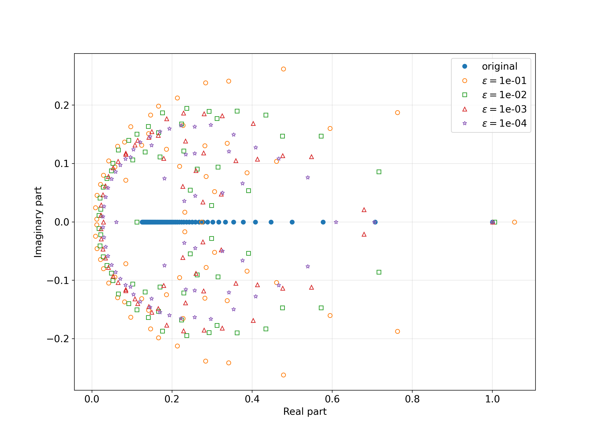
All of the eigenvalues of the original matrix \(A\) are real so they all lie on the real axis. The eigenvalues of the collection of \(A+E\) matrices spread into the imaginary axis. A larger \(\epsilon\) results in larger eigenvalue errors.
The outlier eigenvalue of matrix \(A\) has a value of \(1\). This outlier eigenvalue often plays a significant role in a number of applications. The Arnoldi iteration can extract this value without us having to deal with the actual matrix \(A\) which can be very large. It is essentially a modified Gram-Schmidt process that generates a unitary matrix \(Q\) whose orthogonal columns successively span the Krylov subspace.
After \(n<N\) iterations of the Arnoldi process, we get the following Hessenberg matrix:
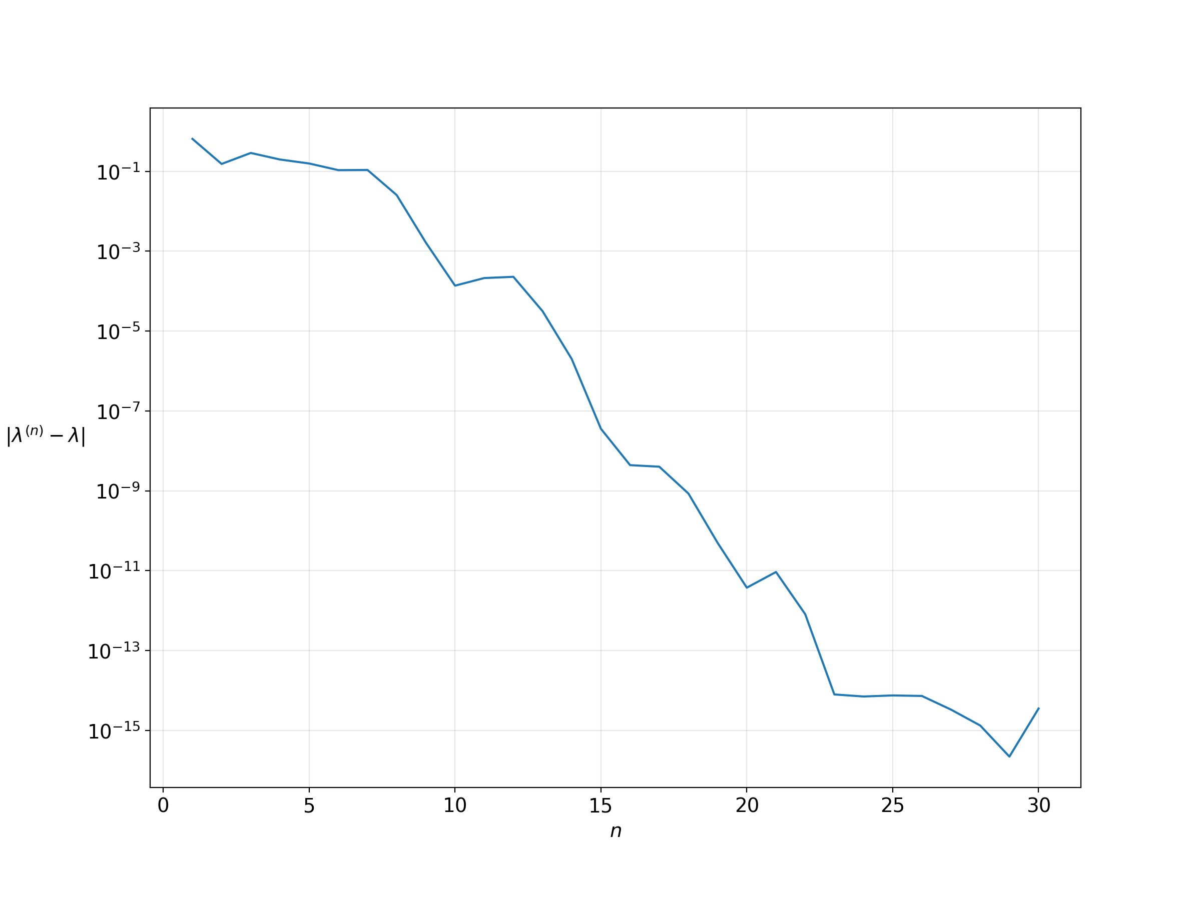
\[H_n = Q^*_nAQ_n\]This Hessenberg matrix is a result of the projection of \(A\) onto \(\mathcal{K_n}\) written with respect to the columns of \(Q_n\). The eigenvalues of \(H_n\) are called Ritz values and their outlier can be a very close approximation of the outlier eigenvalue of \(A\) even though \(n\) is much smaller than \(N\). This is shown in the plot below. The y-axis is the error between the outlier Ritz value \(\lambda^{(n)}\) and the actual outlier eigenvalue \(\lambda\), shown in log scale. The x-axis is the number of Arnoldi iterations. The error decreases rapidly, and we get a very close approximation of the outlier eigenvalue with \(n\) less than half of \(N\).
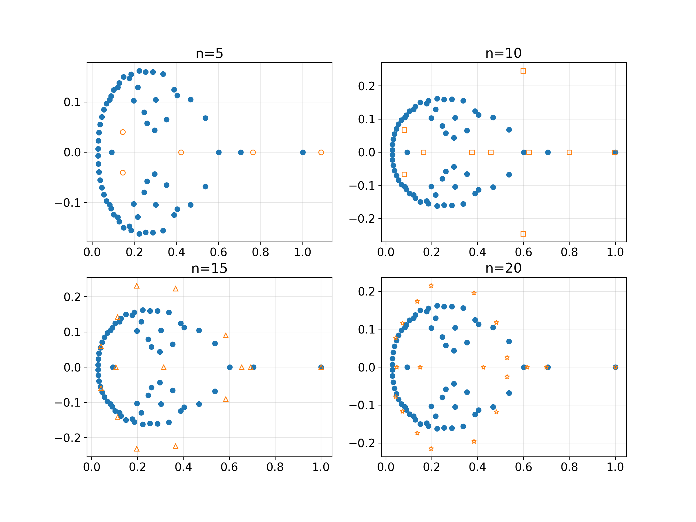
The eigenvalues of \(H_n\) can also approximate the pseudospectra of \(A\). Below is a plot of \(\epsilon\)-pseudospectra where \(\epsilon = 10^{-4}\) compared to the eigenvalues of \(H_n\). A reasonable approximation is obtained at \(n=20\).